Cell Models & Characterisation

Shivaram N V, Gaurav Jain, Hari Vasudevan

In our previous blog post we had described a generic Algorithmic architecture for a BMS that attempts to strike a balance between software maintenance, performance and robustness. In this post we focus on another aspect of BMS algorithm design, namely the characterisation of cell parameters. Estimation of cell parameters is the fundamental building block of any algorithm used in the BMS. The Kalman Filter, the charging and discharge controllers, charging voltage controls etc.. all require knowledge of one or more cell parameters to operate effectively.

If we were to survey the literature for cell models, we would find several models both at the electrolyte/electrode level as well as equivalent circuit /empirical models that approximate the dynamic behaviour of a Li-Ion cell. However while there are descriptions of how to extract the cell parameters from various experiments, no single reference provides a unified guide to extract the cell parameters. In this blog post, we will describe the sequence of steps that are required to extract the cell parameters as well as an example of how to perform this extraction.

Equivalent Circuit Models

Like in any system, modeling of a Lithium ion cell can be done in broadly 3 different ways — White box modeling, Grey box modeling and Black box modeling. White box modeling for a system as complex as an electrochemical cell is extremely hard. It is testing intensive and requires information down to the levels of the quantity and grade of materials used in the cell. Black box modeling lies on the other end of the spectrum where it treats the model purely as a mathematical problem of curve fitting. While this is also testing intensive, the main drawback of this is that at the completion of the curve fitting exercise, you will end up with a black box without any way to infer the impact of change of any parameter not modelled explicitly as inputs or outputs on the system. This is where a Grey box model comes in very handy with a theoretical structure complemented by data to complete the model.

Within the paradigm of Grey box models for Lithium-Ion cells, there are a wide range of models like the Shepherd Model, Unnewehr Universal Model, Nernst Model and the Equivalent Circuit Model. While each of them have their pros and cons vis-à-vis complexity, accuracy, requirements of test data, physical intuition etc., one feature of the Equivalent Circuit Model that we particularly like is the linear ordinary differential equation structure that significantly aids in the process of controller synthesis for charge and discharge controls. Therefore, we recommend the use of the Equivalent Circuit Model for the cell. The equations that define this model are also shown below.

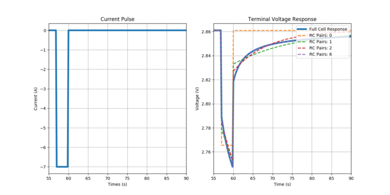
The advantage of a cell model like this is it is generically extensible till the model reaches acceptable performance. Figure 2 demonstrates this. The measured terminal voltage response of a cell for a discharge current pulse is shown by the blue trace, the dashed lines show approximations starting from 0 RC pairs to 6 RC pairs. As we increase the number of RC pairs the response becomes more and more aligned with the measured response. In fact there is virtually no difference between the measured response and the 6 RC pair model response. In fact, even the 2 RC pair model (red trace) could perhaps be an acceptable compromise between the complexity of the model and accuracy. For offline analysis the complexity of the model is not a barrier as compute time available is virtually limitless. However in the scenario where we have to use any of these models in an online iterative algorithm such as a Kalman Filter is where the complexity vs accuracy trade-off needs to be evaluated.

There are of-course drawbacks to the RC parameter model. For example, hysteresis in VOC-SOC table cannot be accurately captured. Coulombic efficiency is similarly hard to model without losing the linearity of the state equation. Despite these drawbacks, the RC model finely treads the line between categories: theoretically accurate but impossible to implement vs. so simple that it does not realistically predict anything. One important point to note here is that the requirements of linearity and ODE structure for the model are mainly for the purpose of observer design and controller synthesis i.e. the Kalman filter and discharge and charge controls. This does not limit one from using a more accurate and computationally complex model as the ‘Plant’ to perform closed loop simulations during the design of the aforementioned observer and controller or for other performance simulations.

Experimental Cell Characterisation

Experimental data under controlled conditions is a crucial part of building the equivalent circuit model. Below we describe the experiments required to derive data points concerning three parameters described in the model. namely, the cell charge capacity (Q), the VOC-SOC curve and the HPPC test to derive the RC parameters.

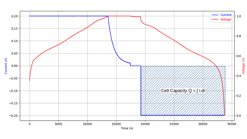
Cell Charge Capacity (Q), generally measured in Ah, is the maximum amount of charge that can be extracted from cell under specific conditions. To measure the cell charge capacity, charge the cell to full. Follow this with a constant current discharge at Qnom/5 Amp till the voltage reaches the end of discharge voltage. Now integrate the value of current through the discharge cycle to get Q (refer Fig 3).
Information on conditions for ‘full charge’ and ‘end of discharge’ are typically provided in cell datasheets. Qnom/5 is the most commonly accepted industry standard for measurement of charge capacity of Li-ion cells. An important point to note here is that while the nominal charge capacity Qnom of the Li-ion cell is provided in most datasheets, what we want to estimate here is the actual capacity Q from a statistically significant number of samples of cells.

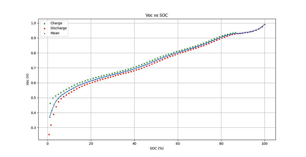
Open Circuit Voltage (Voc) is generally defined as the voltage between the terminals of an electrochemical cell when no current flows through the cell. Low-current Voc and Incremental-current Voc tests are two common methods to observe the VOC-SOC relationship. The Incremental Voc test consists of many SOC intervals and rest periods after which the Voc with the corresponding SOC is measured. The steps required for this test are as given below.

1. Charge cell fully to 100% SOC
2. Discharge at Q/5 using a negative pulse current followed by rest at every x% SOC till end of discharge voltage
3. Charge again following the same routine but with a positive pulse current till end of charge voltage
4. Apply Averaging and Linear Interpolation step to obtain the VOC-SOC curve at different intermediate SOCs

Hybrid pulse power characterisation test, also known as HPPC test. This test investigates the power capabilities of a cell under operating conditions at different temperatures, pulse width and state of charge. The HPPC test based on the defined test sequence provides us the data to derive the RC parameters used in cell model.

• Charge the cell fully to 100% SOC
• After rest, apply constant current discharge and charge pulse of Q/2 Amp for ’n’ seconds and discharge by x% SOC using a pulse of Q/5 Amp with rest in between
• Repeat the same till end of discharge voltage is reached
• Discharge the cell till 0% SOC and repeat the above pulse sequence while charging by x% SOC using charge pulse of Q/5 Amp for measurement during charge
• Repeat the same till end of charge voltage is reached

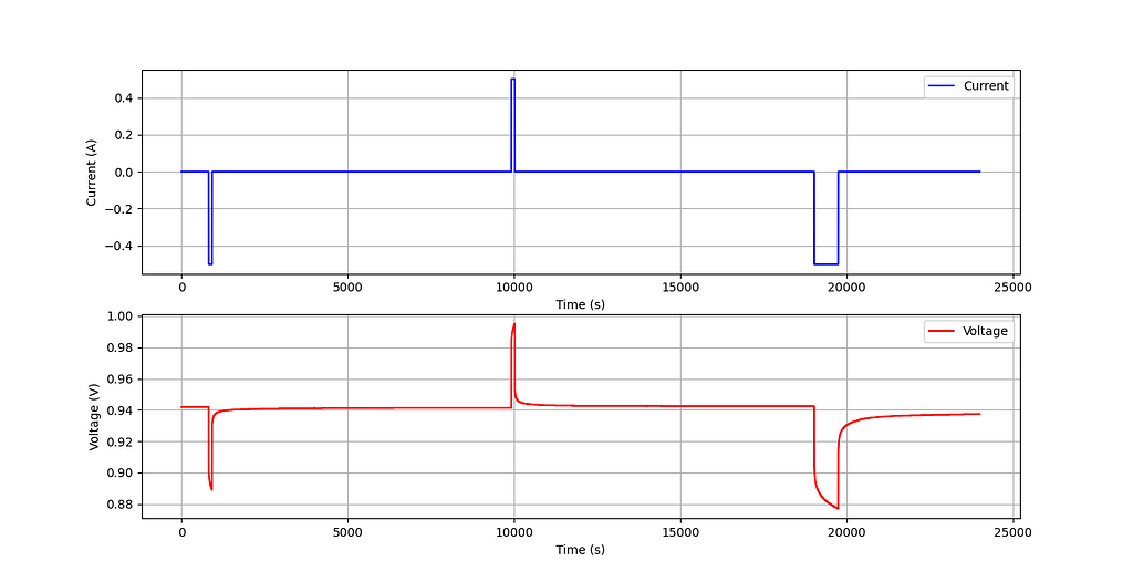
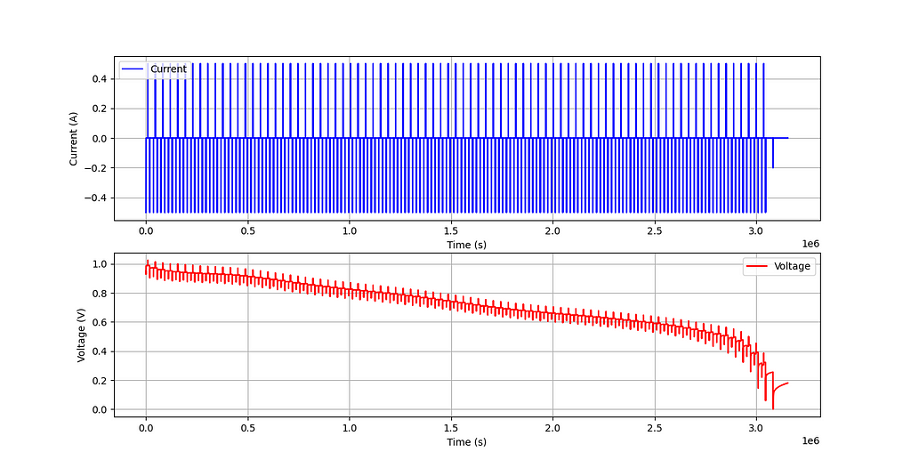
Please note that it can take up to a few hours in rest condition for a cell to return to an electrochemical and thermal equilibrium. Ensuring long rests after charge or discharge pulse improves quality of data. In the next section, we shall see how the data from the above tests can be used to fit the equivalent circuit model.

Parameter Estimation via Convex Optimisation

In the previous section we have described the aspects of cell characterisation as well as the HPPC test. In this section we focus on the extraction of the RC parameters from the HPPC data. Referring back to literature, we see that there are several methods for computing RC parameter values, however these are at best approximations or rules of thumb.

Using the information gathered in the experimental characterisation of the previous section, we can now compute the RC parameters at every SOC measurement point via simple constrained optimisation. In the section below we demonstrate a simple example that computes the RC parameters given an isolated pulse at a particular SOC.

Example

This example illustrates the fundamentals of both simulating the dynamics of a cell model in Python as well as using parameter optimisation to determine RC parameters given the terminal voltage response of a cell to a pulse of current.

First we focus on the cell modelling bit, the code below shows how parameters obtained from cell testing can be organised to create a dynamic model of the cell. Please note that here the RC parameters are described at a certain SOC. In reality however, the RC parameters values vary with SOC and must be defined at every SOC point. Nevertheless this is a good starting point.

To define a cell we have to define the following parameters

• Cell Capacity
• VOC vs SOC Table
• RC Model Parameters

The loadCellFn defines these parameters for use in the simulation as well as the RC parameters for a particular SOC. As mentioned earlier, RC parameters are not constant and change as a function of SOC. However for now we are going to ignore this fact.

https://medium.com/media/22f780842ccf204327ecfbf3dcd9e9bd/href

We now define a current pulse that is an input to the cell model. The code snippet below constructs this pulse at a defined sampling rate.

https://medium.com/media/184694d0c7d0ff449be68f1f798a9cef/href

Now comes the fun part. Using Equation 1 we can define the cell model in Python and then use the lsim function to model the behaviour of the cell given the current pulse input. Please note that we can use lsim for this because the state equation defined by Equation 1 is linear where as the measurement equation defined by Equation 2 is non linear. If this was not the case we would have to use the odeint function to solve the non-linear dynamic equations. Finally after invoking lsim the output terminal voltage “Vt” is then computed using the nonlinear measurement equations. The results are also plotted at the end of the gist snippet below.

https://medium.com/media/a8792e6f3ec38af9dd2c1fbd81663a3a/href

For this hypothetical cell, we use a higher order model (10 RC Pair) response as the measured data (Full Cell Response) for performing the optimisation. We then demonstrate how to compute the values RC parameters for lower order models. Note that this is similar to real life situations where the result of the HPPC test is used to fit the RC parameters. To do this we use least squares fitting using the SciPy minimise function. The minimise function iterates over RC parameter values using the default solver, note that we have the choice of selecting different solvers or different fit criteria to ensure that the results are more inline with our measured data, the further tweaking of the solver is not considered for this blog post. The gist shown below provides a code snippet for this optimisation.

https://medium.com/media/34e29bab1ec9d518f139c75a859743eb/href

The following figures show the evolution of the RC parameters in every iteration of the solver and the final best fit. Note that with 6-RC pairs we obtain an the almost exact response of the 10-RC pair model. In a real life scenario we would only model a 6 -RC pair network to save ourselves the computational complexity of a 10-RC pair model.

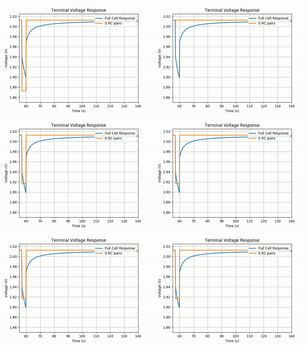
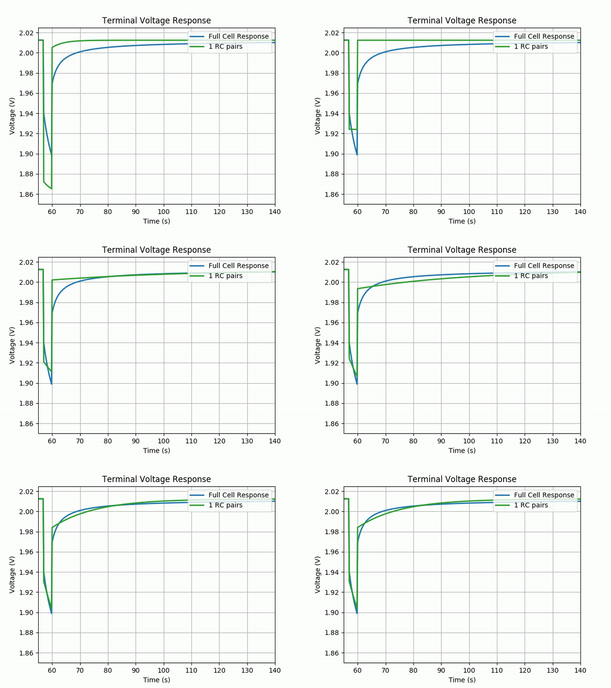
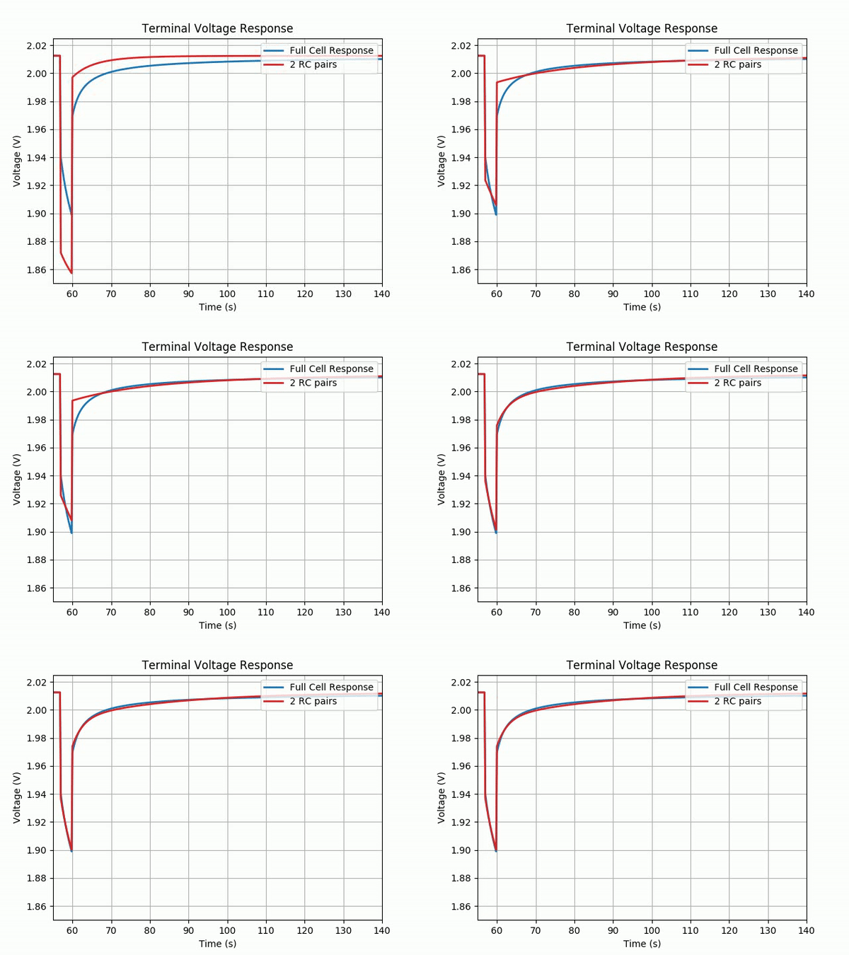
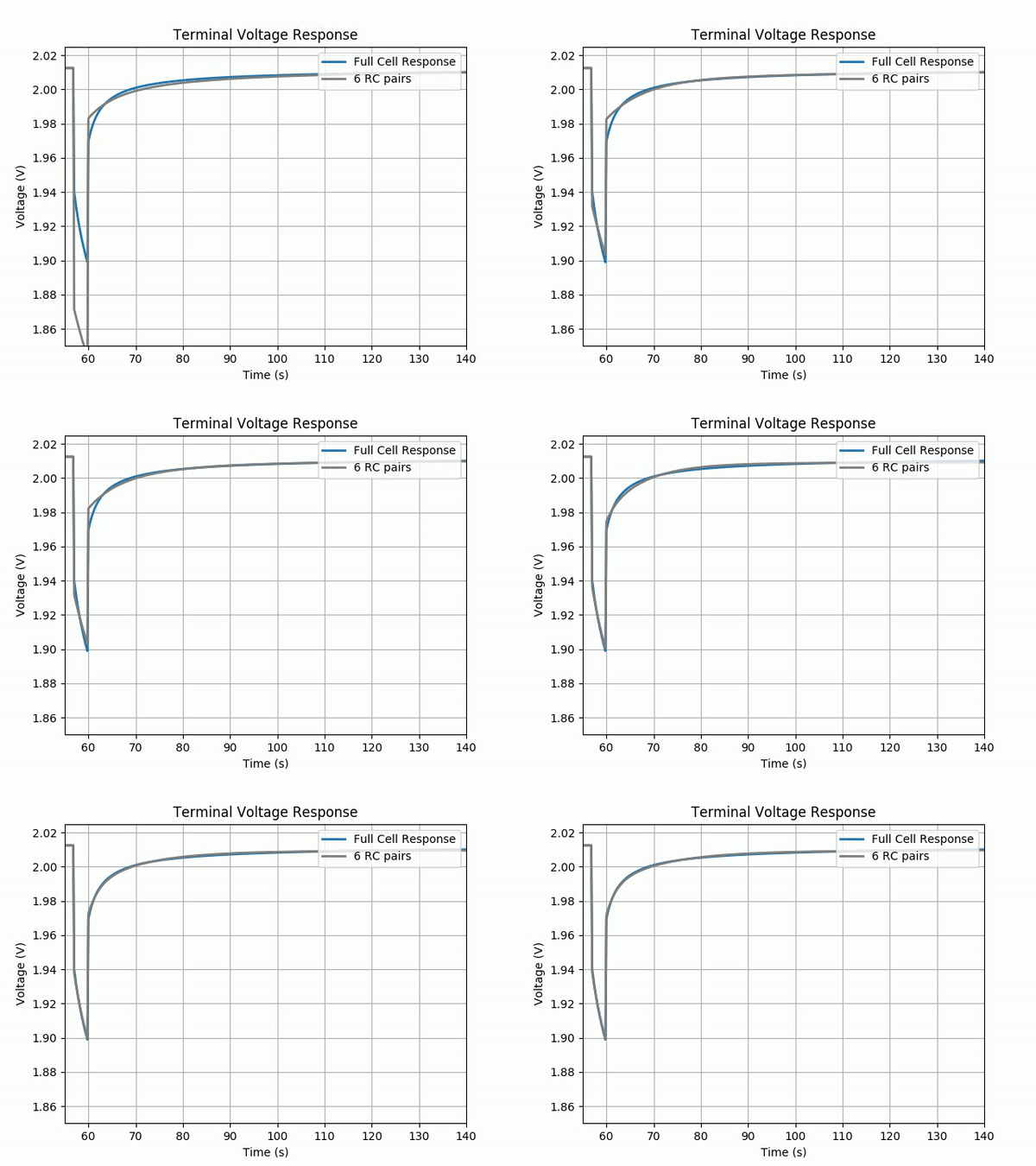
The code to perform both the cell modelling and the RC parameter estimation is given in the snippet below. Try to change the RC parameter values and/or the optimisation parameters to view effects on the parameter estimation and how it effects the final fit.

https://medium.com/media/80ff99c6d4ebb5a39d53f4360b194de2/href

Conclusions and Inference

In the sections above we have seen how we can start with an equivalent cell model and gradually build up enough experimental data and code to derive the appropriate parameters for a Lithium ion cell. While this gives an introductory idea on how to characterise a cell for use in EVs, there are several complexities we have glossed over. These include:

• The effect of temperature
• The effects of VOC-SOC Hysteresis
• Validity of the model at edges of SOC, i.e typically less than 2% or greater then 98% SOC
• Issues with the Convex Optimisation solver at various SOC points, i.e how to keep the RC values smoother and now have them arbitrarily swap places

As part of these series of blogs, we will next focus on the construction and implementation of an Extended Kalman Filter (EKF) for EV applications and the constraints imposed on the tuning of the EKF due to user-facing requirements. Stay tuned for more on this…

References

• Lectures by Dr. Gregory L. Plett -University of Colorado Colorado Springs -ECE5720: Equivalent-Circuit Cell Models — Notes 2
• An Overview of Generic Battery Models -https://www.researchgate.net/publication/327222260_An_Overview_of_Generic_Battery_Models

Cell Models & Characterisation was originally published in Ather Energy on Medium, where people are continuing the conversation by highlighting and responding to this story.